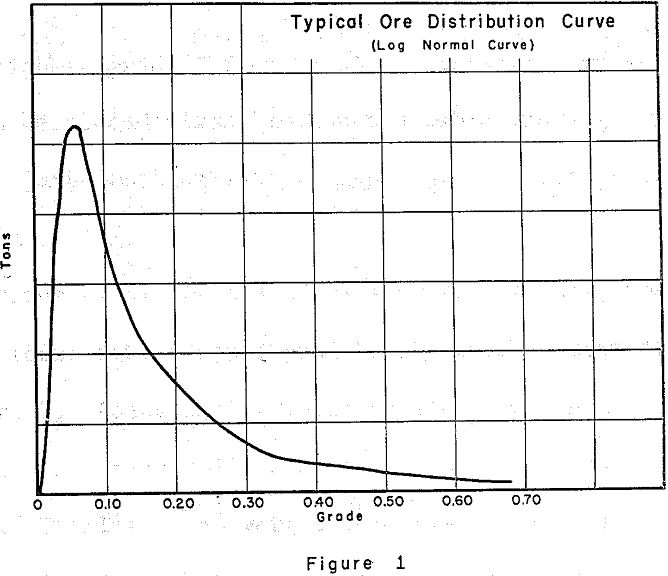
There are certain data handling techniques used by statisticans that can help one to calculate the size of an orebody and to develop some of the relationships between size, cutoff grade, average grade, mining cost, and profit. Knowing the relationships amongst these factors can help determine the most desirable operating conditions.
A statistical technique that we will use is data grouping. This allows us to work with relatively few groups instead of many samples. If we were able to segregate the ore in an orebody into grade groups, add the amounts in each group, and plot the sums as a curve. A smooth curve develops when the grade classes are small enough, otherwise a “stair step” histogram results. The area under the curve, being the sum of the tonnages in all of the grade classes, is proportional to the total number of tons in the orebody.
A simplification can be made to give us a workable technique. Sampling of orebodies, either by drilling or underground sampling, can often be performed in such a way that each sample has an equal area of influence. This condition would be satisfied by sampling performed on a uniform grid pattern or by a system of random sample spacings such that there is small variation in the areas represented by the samples. For random spacing, area variation is less critical if the orebody is fairly uniform in thickness and grade. With equal areas of influence, tonnage is proportional to the thickness. This dimension is determined from the sample representing the area. Each foot of sample length will represent the same tonnage; an amount equal to the area of influence divided by the tonnage factor in cubic feet per ton. Thus we can use sample lengths directly to analyze an orebody.

As a practical consideration a 5-foot minimum working height was assumed for this: calculation. To meet this requirement we averaged
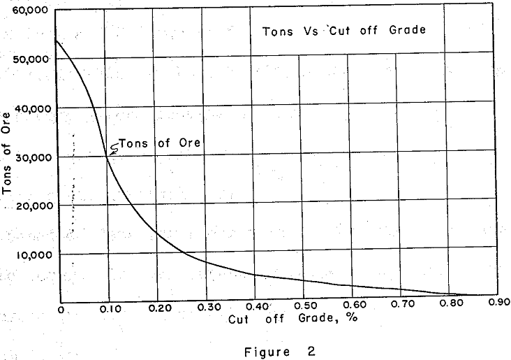

After grouping all of the samples of the orebody, the columns are totaled. Accumulating these totals from the highest grade bracket down to the lowest will produce the total footage above any of the grades. Finally we convert our footage of sample lengths to tonnages by multiplying by the appropriate factor. In our example we arbitrarily use 200 tons per foot of sample length.
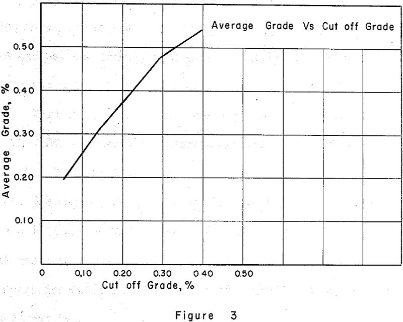
Plotting the average grades thus calculated for our example against cutoff grades. This graph tells us the average grade that will result if we select any particular cutoff, conversely, the cutoff we need to use if we desire a certain average grade. Using these curves we see that the character of our orebody is such that a 0.10% cutoff results in a 30,000 ton orebody with an average grade of 0.25% whereas a cutoff of 0.20% results in an orebody of 14,000 tons averaging 0.37%.
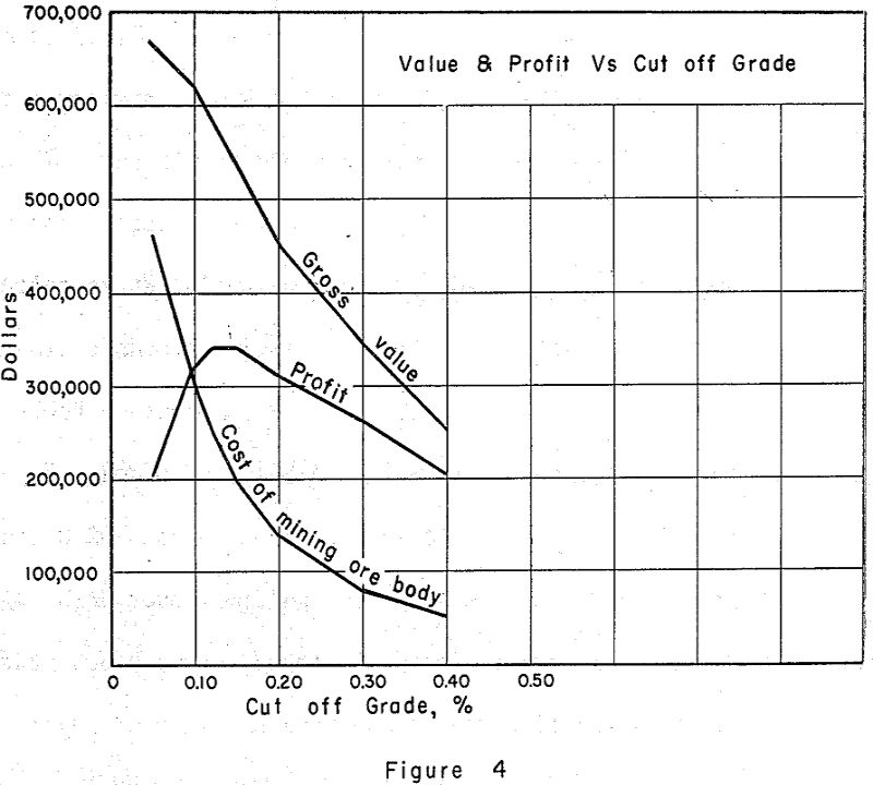
To decide which of the many combinations of tonnage and grade we will finally use, we must turn to dollars and cents. Since we know the tons and grade for each cutoff, we can calculate the gross value of the ore. The upper curve in Figure 4 shows how these values work out for our example if the grades were for U3O8 and price is determined by AEC Circular 5.
Dilution will decrease profit as ore is converted to a grade lower than is desired and increased tonnages are handled.
