Table of Contents
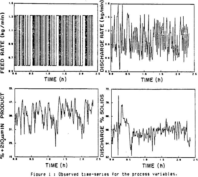
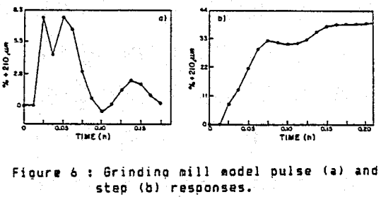
Dynamic experiments were performed in a continuous open-circuit 40×40 cm ball mill using a pseudo-random binary sequence of the feed rate and measuring the variations of the discharge particle-size distribution. The impulse response is calculated by a cross- correlation technique. Then a model involving a discrete transfer function and a time-series stochastic equation is calibrated using maximum likelihood methods.
Experimental
A continuous grinding experiment is performed in a Denver 40 x 40 cm grate discharge ball mill. The mill feed (quartz in the range of 600-1700 um) is delivered by a PI-controlled belt conveyor accurate to ±1%. The water addition to the mill is automatically adjusted by a peristaltic pump to maintain a constant percentage of solids in the feed (65%). A PDP 11/23 mini-computer is used for remote set-points control.
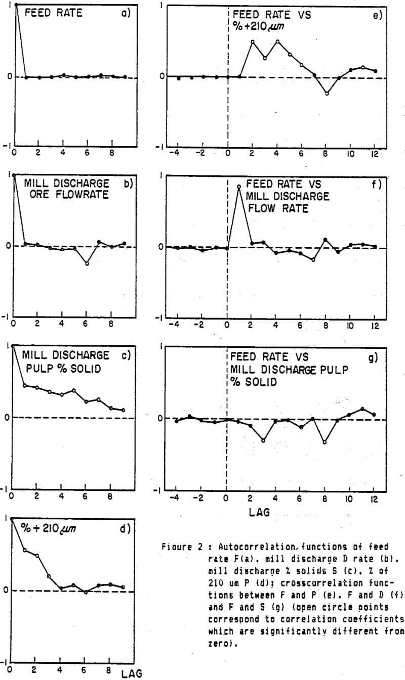
Fiaure 2 gives the auto and crosscorrelation functions of the various measured variables of the grinding test. The autocorrelograms show that both ore feed and discharge rates are white. This was expected for the feed rate since a PRBS was used. The results for the mill discharge rate indicate that the dynamic behaviour of the mill load is faster than the sampling period, i.e. that the mill solids hold-up weight reaches an equilibrium within 45 seconds after a feed rate variation.
Grinding mill modelling
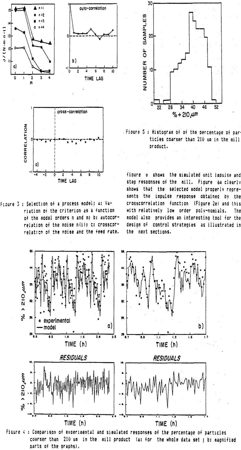
The studied model relates dynamically the mill discharge product size P to the mill feed rate F. Since the sampling interval is too large to characterize the dynamics of the mill discharge rate and percentage of solids, the models for these two variables are not considered here.
The model structure used is a discrete transfer function of the form:
![]()
which relates a deterministic output variable v(i) observed at the sampling interval i, to an input variable u(i). The polynomials A(z-¹) and B(z-¹) are:

where z-¹ is the backshift operator.
The residuals together with the observed and deterministic process outputs, are in this particular case mainly due to measurement (sampling and analysis) errors. However they have not a zero mean, since the model is unable to represent the unequal distribution at the experimental points around the mean value of P which is observed in the assymetrical shape of the P histogram.
Constrained minimum variance control
A possible approach for limiting the variability of the manipulated variable is to estimate u(i) such that the weighted sum of the variances of u(i) and e(i) is minimum. This leads to the well-known Linear-Quadratic-Gaussian (LQG) control. Another approach, known as the “one-step ahead” MV controller yields a sub-optimal control law without the complicated mathematics of the LOG.
This study shows that it is possible with appropriate experiments to find a dynamic linear empirical model of a continuous grinding ball mill the advantage of empirical modelling compared to phenomenological modelling is its ability to represent the experimental facts as they are without forcing them to obey a preconceived model structure. The universal structure of the model is an other advantage which gives access to the standard mathematical tools for process identification and control.
Illustrations of this point are given by the application of the maximum likelihood method to the estimation of the mill model parameters and the application of the minimum variance control theory to the control of the product fineness by the ore feed rate. It is shown by simulation that, for different types or minimum variance controllers and different types of disturbances, the MV controller exhibits better performances than an optimally tuned PID controller. However it is very demanding for the actuators and can lead to irrealistic or unstable control laws. The “one-step ahead” MV controller exhibits a safer behaviour than the unconstrained MV controller since it allows a flexible limitation of the feed rate variations. When the product fineness disturbances are strongly non-stationary, it is shown that a constraint on the feed rate variation between successive values is very efficient to eliminate the controller offset and reduce the oscillation of the feed rate.
The empirical approach to grinding modelling and control presents also some implementation difficulties. First of all since the process model unavoidly changes with time, it must be estimated by adaptive methods such as it is in self-tuning controllers. Second the MV controller requires the knowledge of the
The disturbances model; which has to be identified by off-line or on-line estimation procedures. Furthermore, when the disturbances model structure changes the MV controller becomes less efficient than the PID controller. Again, adaptive procedures are required to track the noise model. Finally when the structure of the randomly occuring deterministic disturbances is different from the stochastic disturbances structure (related for instance to measurement inaccuracies), more elaborate control strategies based on state-space formulation have to be considered.